This article introduces the concepts of risk and uncertainty together with techniques which are used for decision-making. In the Professional Diploma in Sustainability, it is unlikely that candidates will be presented with complex risk and uncertainty calculations but understanding the techniques can be helpful when responding to questions on risk management more generally.
Clearly, risk permeates most aspects of corporate decision-making (and life in general), and few can predict with any precision what the future holds in store.
Risk can take myriad forms – ranging from the specific risks faced by individual companies (such as financial risk, or the risk of a strike among the workforce), through the current risks faced by particular industry sectors (such as banking, car manufacturing, or construction), to more general economic risks resulting from interest rate or currency fluctuations, and, ultimately, the looming risk of economic recession. Risk often has negative connotations, in terms of potential loss, but the potential for greater than expected returns also often exists.
Clearly, risk is almost always a major variable in real-world corporate decision-making, and managers ignore its vagaries at their peril. Similarly, accountants require an ability to identify the presence of risk and incorporate appropriate adjustments into the problem-solving and decision-making scenarios encountered. While it is unlikely that precise probabilities and perfect information, which feature in examinations can be transferred to real-world scenarios, a knowledge of the relevance and applicability of such concepts is necessary.
The basic definition of risk is that the final outcome of a decision, such as an investment, may differ from that which was expected when the decision was taken. We tend to distinguish between risk and uncertainty in terms of the availability of probabilities. Risk is when the probabilities of the possible outcomes are known (such as when tossing a coin or throwing a dice); uncertainty is where the randomness of outcomes cannot be expressed in terms of specific probabilities. However, it has been suggested that in the real world, it is generally not possible to allocate probabilities to potential outcomes, and therefore the concept of risk is largely redundant.
Probability
The term ‘probability’ refers to the likelihood or chance that a certain event will occur, with potential values ranging from 0 (the event will not occur) to 1 (the event will definitely occur). For example, the probability of a tail occurring when tossing a coin is 0.5, and the probability when rolling a dice that it will show a four is 1/6 (0.166). The total of all the probabilities from all the possible outcomes must equal 1 – i.e. some outcome must occur.
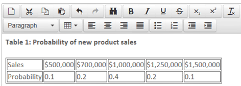
A real-world example could be that of a company forecasting potential future sales from the introduction of a new product in year one (Table 1).

From Table 1, it is clear that the most likely outcome is that the new product generates sales of £1,000,000, as that value has the highest probability.
Independent and conditional events
An independent event occurs when the outcome does not depend on the outcome of a previous event. For example, assuming that a dice is unbiased, then the probability of throwing a five on the second throw does not depend on the outcome of the first throw.
In contrast, with a conditional event, the outcomes of two or more events are related – i.e. the outcome of the second event depends on the outcome of the first event. For example, in Table 1, the company is forecasting sales for the first year of the new product. If, subsequently, the company attempted to predict the sales revenue for the second year, then it is likely that the predictions made will depend on the outcome for year one. If the outcome for year one was sales of $1,500,000, then the predictions for year two are likely to be more optimistic than if the sales in year one were $500,000.
The availability of information regarding the probabilities of potential outcomes allows the calculation of both an expected value for the outcome, and a measure of the variability (or dispersion) of the potential outcomes around the expected value (most typically standard deviation). This provides us with a measure of risk which can be used to assess the likely outcome.
Expected values and dispersion
Using the information regarding the potential outcomes and their associated probabilities, the expected value of the outcome can be calculated simply by multiplying the value associated with each potential outcome by its probability. Referring back to Table 1, regarding the sales forecast, then the expected value of the sales for year one is given by:
Expected value
= ($500,000 x 0.1) + ($700,000 x 0.2) + ($1,000,000 x 0.4) + ($1,250,000 x 0.2) + ($1,500,000)(0.1)
= $50,000 + $140,000 + $400,000 + $250,000 + $150,000
= $990,000
In this example, the expected value is very close to the most likely outcome, but this is not necessarily always the case. Moreover, it is likely that the expected value does not correspond to any of the individual potential outcomes. For example, the average score from throwing a dice is (1 + 2 + 3 + 4 + 5 + 6) / 6 or 3.5. A further point regarding the use of expected values is that the probabilities are based upon the event occurring repeatedly, whereas, in reality, most events only occur once.
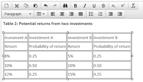
In addition to the expected value, it is also informative to have an idea of the risk or dispersion of the potential actual outcomes around the expected value. The most common measure of dispersion is standard deviation (the square root of the variance), which can be illustrated by the example given in Table 2, concerning the potential returns from two investments.

To estimate the standard deviation, we must first calculate the expected values of each investment:
Investment A
Expected value = (8% x 0.25) + (10% x 0.5) + (12% x 0.25) = 10%
Investment B
Expected value = (5% x 0.25) + (10% x 0.5) + (15% x 0.25) = 10%
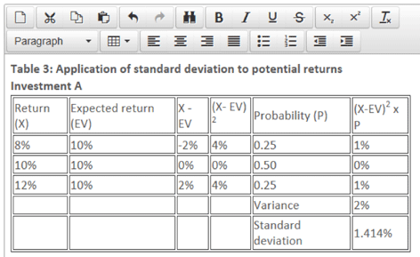
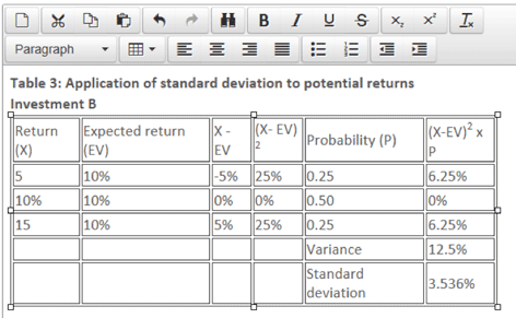
The calculation of standard deviation proceeds by subtracting the expected value from each of the potential outcomes, then squaring the result and multiplying by the probability. The results are then totalled to yield the variance and, finally, the square root is taken to give the standard deviation, as shown in Table 3.


In Table 3, although investments A and B have the same expected return, investment B is shown to be riskier by exhibiting a higher standard deviation. More commonly, the expected returns and standard deviations from investments and projects are both different, but they can still be compared by using the coefficient of variation, which combines the expected return and standard deviation into a single figure.
Coefficient of variation and standard error
The coefficient of variation is calculated simply by dividing the standard deviation by the expected return (or mean):
Coefficient of variation = standard deviation / expected return
For example, assume that investment X has an expected return of 20% and a standard deviation of 15%, whereas investment Y has an expected return of 25% and a standard deviation of 20%. The coefficients of variation for the two investments will be:
Investment X = 15% / 20% = 0.75
Investment Y = 20% / 25% = 0.80
The interpretation of these results would be that investment X is less risky, on the basis of its lower coefficient of variation. A final statistic relating to dispersion is the standard error, which is a measure most often confused with standard deviation. Standard deviation is a measure of variability of a sample, used as an estimate of the variability of the population from which the sample was drawn. When we calculate the sample mean, we are usually interested not in the mean of this particular sample, but in the mean of the population from which the sample comes. The sample mean will vary from sample to sample and the way this variation occurs is described by the ‘sampling distribution’ of the mean. We can estimate how much a sample mean will vary from the standard deviation of the sampling distribution. This is called the standard error (SE) of the estimate of the mean.
The standard error of the sample mean depends on both the standard deviation and the sample size:
SE = SD/√(sample size)
The standard error decreases as the sample size increases, because the extent of chance variation is reduced. However, a fourfold increase in sample size is necessary to reduce the standard error by 50%, due to the square root of the sample size being used. By contrast, standard deviation tends not to change as the sample size increases.
Bayes' rule
Bayes' rule is perhaps the preferred method for estimating revised (posterior) probabilities when imperfect information is available. An intuitive introduction to Bayes' rule was provided in The Economist, 30 September 2000:
'The essence of the Bayesian approach is to provide a mathematical rule explaining how you should change your existing beliefs in the light of new evidence. In other words, it allows scientists to combine new data with their existing knowledge or expertise. The canonical example is to imagine that a precocious newborn observes his first sunset, and wonders whether the sun will rise again or not. He assigns equal prior probabilities to both possible outcomes and represents this by placing one white and one black marble into a bag. The following day, when the sun rises, the child places another white marble in the bag. The probability that a marble plucked randomly from the bag will be white (i.e. the child's degree of belief in future sunrises) has thus gone from a half to two-thirds. After sunrise the next day, the child adds another white marble, and the probability (and thus the degree of belief) goes from two-thirds to three-quarters. And so on. Gradually, the initial belief that the sun is just as likely as not to rise each morning is modified to become a near-certainty that the sun will always rise.'
In mathematical terms, Bayes' rule can be stated as:
| Posterior probability = | likelihood x prior probability marginal likelihood |
For example, consider a medical test for a particular disease which is 90% accurate, i.e. if you test positive then there is a 90% probability that you have the disease and a 10% probability that you have been misdiagnosed. If we further assume that 3% of the population actually have this disease, then the probability of having the disease (given that you have tested positive) is shown by:
P(Disease|Test = +) =
P(Test = +|Disease) x P(Disease)
P(Test = +|Dis) x P(Dis) + P(Test= +|No Dis) x P(No Dis)
= 0.90 0.03; 0.027;
0.90 x 0.03 + 0.10 x 0.97 0.027 + 0.097
= 0.218
This result suggests that you have a 22% probability of having the disease, given that you tested positive. This may seem a low probability but only 3% of the population have the disease and we would expect them to test positive. However, 10% of tests will prove positive for people who do not have the disease. Therefore, if 100 people are tested, approximately three out of the 13 positive tests will actually have the disease.
Bayes' rule has been used in a practical context for classifying email as spam on the basis of certain key words appearing in the text.
Value-at-Risk (VaR)
Although financial risk management has been a concern of regulators and financial executives for a long time, Value-at-Risk (VaR) did not emerge as a distinct concept until the late 1980s. The triggering event was the stock market crash of 1987, which was so unlikely, given standard statistical models, that it called the entire basis of quantitative finance into account.
VaR is a widely used measure of the risk of loss on a specific portfolio of financial assets. For a given portfolio, probability, and time horizon, VaR is defined as a threshold value such that the probability that the mark-to-market loss on the portfolio over the given time horizon exceeds this value (assuming normal markets and no trading) is the given probability level. Such information can be used to answer questions such as 'What is the maximum amount that I can expect to lose over the next month with 95%/99% probability?'
For example, large investors, interested in the risk associated with the FT100 index, may have gathered information regarding actual returns for the past 100 trading days. VaR can then be calculated in three different ways:
1. The historical method
This method simply ranks the actual historical returns in order from worst to best, and relies on the assumption that history will repeat itself. The largest five (one) losses can then be identified as the threshold values when identifying the maximum loss with 5% (1%) probability.
2. The variance-covariance method
This relies upon the assumption that the index returns are normally distributed, and uses historical data to estimate an expected value and a standard deviation. It is then a straightforward task to identify the worst 5 or 1% as required, using the standard deviation and known confidence intervals of the normal distribution - i.e. -1.65 and -2.33 standard deviations respectively.
3. Monte Carlo simulation
While the historical and variance-covariance methods rely primarily upon historical data, the simulation method develops a model for future returns based on randomly generated trials.
Admittedly, historical data is utilised in identifying possible returns but hypothetical, rather than actual, returns provide the data for the confidence levels.
Of these three methods, the variance-covariance is probably the easiest as the historical method involves crunching historical data and the Monte Carlo simulation is more complex to use.
VaR can also be adjusted for different time periods, since some users may be concerned about daily risk whereas others may be more interested in weekly, monthly, or even annual risk. We can rely on the idea that the standard deviation of returns tends to increase with the square root of time to convert from one time period to another. For example, if we wished to convert a daily standard deviation to a monthly equivalent then the adjustment would be:
σ monthly = σ daily x √T where T = 20 trading days
For example, assume that after applying the variance-covariance method we estimate that the daily standard deviation of the FT100 index is 2.5%, and we wish to estimate the maximum loss for 95 and 99% confidence intervals for daily, weekly, and monthly periods assuming five trading days each week and four trading weeks each month:
95% confidence
Daily = -1.65 x 2.5% = -4.125%
Weekly = -1.65 x 2.5% x √5 = -9.22%
Monthly = -1.65 x 2.5% x √20 = -18.45%
99% confidence
Daily = -2.33 x 2.5% = -5.825%
Weekly = -2.33 x 2.5% x √5 = -13.03%
Monthly = -2.33 x 2.5% x √20 = -26.05%
Therefore, we could say with 95% confidence that we would not lose more than 9.22% per week, or with 99% confidence that we would not lose more than 26.05% per month.
On a cautionary note, New York Times reporter Joe Nocera published an extensive piece entitled Risk Mismanagement on 4 January 2009, discussing the role VaR played in the ongoing financial crisis. After interviewing risk managers, the author suggests that VaR was very useful to risk experts, but nevertheless exacerbated the crisis by giving false security to bank executives and regulators. A powerful tool for professional risk managers, VaR is portrayed as both easy to misunderstand, and dangerous when misunderstood.
Conclusion
These two articles have provided an introduction to the topic of risk present in decision making, and the available techniques used to attempt to make appropriate adjustments to the information provided. Adjustments and allowances for risk also appear elsewhere in the ACCA syllabus, such as sensitivity analysis, and risk-adjusted discount rates in investment appraisal decisions where risk is probably at its most obvious. Moreover, in the current economic climate, discussion of risk management, stress testing and so on is an everyday occurrence.
References
- Jorion, P (2006), Value at Risk: The New Benchmark for Managing Financial Risk, 3rd edition, McGraw Hill
- Nocera, J (2009), Risk Management, New York Times
- Taleb, N (2007), Black Swan, Random House Publishing
Adapted from an article written by a member of the Advanced Performance Management examining team


