Time series analysis can be used to analyse historic data and establish any underlying trend and seasonal variations within the data. The trend refers to the general direction the data is heading in and can be upward or downward. The seasonal variation refers to the regular variations which exist within the data. This could be a weekly variation with certain days traditionally experiencing higher or lower sales than other days, or it could be monthly or quarterly variations.
The trend and seasonal variations can be used to help make predictions about the future – and as such can be very useful when budgeting and forecasting.
Calculating moving averages
One method of establishing the underlying trend (smoothing out peaks and troughs) in a set of data is using the moving averages technique. Other methods, such as regression analysis can also be used to estimate the trend. Regression analysis is dealt with in a separate article.
A moving average is a series of averages, calculated from historic data. Moving averages can be calculated for any number of time periods, for example a three-month moving average, a seven-day moving average, or a four-quarter moving average. The basic calculations are the same.
The following simplified example will take us through the calculation process.
Monthly sales revenue data were collected for a company for 20X2:
| Jan | Feb | Mar | Apr | May | Jun | Jul | Aug | Sep | Oct | Nov | Dec | |
| Sales $000 | 125 | 145 | 186 | 131 | 151 | 192 | 137 | 157 | 198 | 143 | 163 | 204 |
From this data, we will calculate a three-month moving average, as we can see a basic cycle that follows a three-monthly pattern (increases January – March, drops for April then increases April – June, drops for July and so on). In an exam, the question will state what time period to use for this cycle/pattern in order to calculate the averages required.
Step 1 – Create a table
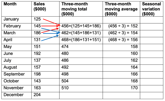
Create a table with 5 columns, shown below, and list the data items given in columns one and two. The first three rows from the data given above have been input in the table:

Step 2 – Calculate the three-month moving average.
Add together the first three sets of data, for this example it would be January, February and March. This gives a total of (125+145+186) = 456. Put this total in the middle of the data you are adding, so in this case across from February. Then calculate the average of this total, by dividing this figure by 3 (the figure you divide by will be the same as the number of time periods you have added in your total column). Our three-month moving average is therefore (456 ÷ 3) = 152.

The average needs to be calculated for each three-month period. To do this you move your average calculation down one month, so the next calculation will involve February, March and April. The total for these three months would be (145+186+131) = 462 and the average would be (462 ÷ 3) = 154.

Continue working down the data until you no longer have three items to add together. Note: you will have fewer averages than the original observations as you will lose the beginning and end observations in the averaging process.
Step 3 – Calculate the trend
The three-month moving average represents the trend. From our example we can see a clear trend in that each moving average is $2,000 higher than the preceding month moving average. This suggests that the sales revenue for the company is, on average, growing at a rate of $2,000 per month.
This trend can now be used to predict future underlying sales values.
Step 4 – Calculate the seasonal variation
Once a trend has been established, any seasonal variation can be calculated. The seasonal variation can be assumed to be the difference between the actual sales and the trend (three-month moving average) value. Seasonal variations can be calculated using the additive or multiplicative models.
Using the additive model:
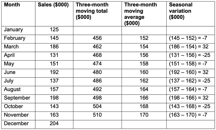
To calculate the seasonal variation, go back to the table and for each average calculated, compare the average to the actual sales figure for that period.

A negative variation means that the actual figure in that period is less than the trend and a positive figure means that the actual is more than the trend.
From the data we can see a clear three-month cycle in the seasonal variation. Every first month has a variation of -7, suggesting that this month is usually $7,000 below the average. Every second month has a variation of 32 suggesting that this month is usually $32,000 above the average. In month 3, the variation suggests that every third month, the actual will be $25,000 below the average.
It is assumed that this pattern of seasonal adjustment will be repeated for each three-month period going forward.
Using the multiplicative model:
If we had used the multiplicative model, the variations would have been expressed as a percentage of the average figure, rather than an absolute. For example:

This suggests that month 1 is usually 95% of the trend, month 2 is 121% and month 3 is 84%. The multiplicative model is a better method to use when the trend is increasing or decreasing over time, as the seasonal variation is also likely to be increasing or decreasing.
Note that with the additive model the three seasonal variations must add up to zero (32-25-7 = 0). Where this is not the case, an adjustment must be made. With the multiplicative model the three seasonal variations add to three (0.95 + 1.21 + 0.84 = 3). (If it was four-month average, the four seasonal variations would add to four etc). Again, if this is not the case, an adjustment must be made.
In this simplified example the trend shows an increase of exactly $2,000 each month, and the pattern of seasonal variations is exactly the same in each three-month period. In reality a time series is unlikely to give such a perfect result.
Step 5 – Using time series to forecast the future
Now that the trend and the seasonal variations have been calculated, these can be used to predict the likely level of sales revenue for the future.
Question:
Using the above example, what is the predicted level of sales revenue for June 20X3 and July 20X3?
Solution:
Start with the trend then apply the seasonal variations. We calculated an increasing trend of $2,000 per month. The last figure we calculated was for November 20X2 showing $170,000. If we assume the trend continues as it has done previously, then by June 20X3, the sales revenue figure will have increased by $14,000 ($2,000 per month for seven months). Adding this to the figure we have for November, we can predict the underlying trend value for June 20X3 to be $184,000. ($14,000 + $170,000).
We know that sales exhibit a seasonal variation. Taking account of the seasonal variation will give us a better estimate for June 20X3. From the table in step 4, we can see that June has a positive variation of $32,000.
Our estimate for the sales revenue for June 20X3 is therefore $184,000 + $32,000 = $216,000.
For July, the underlying trend value will be $170,000 + $16,000 = $186,000. The seasonal variation for July 20X3 is a negative variation of $25,000, therefore our estimate for the sales revenue for July 20X3 is $186,000 - $25,000 = $161,000.
Calculating moving averages for an even number of periods
In the above example, we used a three-month moving average. Looking back at step 2, we can see that the average is shown against the mid-point of the three observations. The mid-point of the period for January, February and March is shown against the February observation.
When we are calculating a moving average with an even number of periods, for example a four-quarter moving average, we do the same basic calculation, but the mid-point will lie between observations. From step 4 above, we can see that we need the moving average to be shown against an observation so that the seasonal variation can be calculated. We therefore calculate the four-quarter moving average as before, but we then calculate a second moving average.
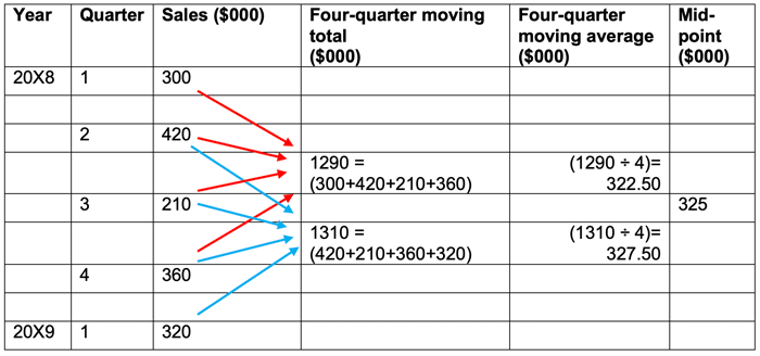
In the example below, the four-quarter moving averages have been calculated in the same way as before. The first four observations are added together and then divided by four. The four-quarter moving average for the first four quarters is 322.50. Moving to the next four observations, gives an average of 327.50. We can then work out the mid-point of these two averages by adding them together and dividing by two. This gives a mid-point of (322.50 + 327.50) ÷ 2 = 325. This mid-point is our trend and the figure is shown against the quarter 3, 20X8 observation. All other calculations are done in the same way as our original example.

Conclusion
Care must be taken however when using time series analysis. This forecasting method is based on the assumption that what has happened in the past is a good indicator of what is likely to happen in the future. In this example the suggestion is that sales revenue will continue to grow by $2,000 per month indefinitely. If we consider the concept of the product lifecycle, we can see that this is a rather simplistic and flawed assumption.
In the real world, changes in the environment (technological, social, environmental, political, economic etc) can all create uncertainty, making forecasts made from past observations unrealistic.
Written by a member of the Performance Management examining team


